Introduction
If you’re familiar with Pandas, this won’t be news to you, but if not, I hope you’ll read through this and be convinced to check Pandas out. Many of us wrestle with data, whether at work, at home, or in our hobbies. If we’re doing robotics or software, there’s almost certain to be logs of data to analyze. Excel is the go to choice for many, and it’s quite useful, but it’s not easy to automate reading in data, reformatting it as you need it, maybe resampling the data, etc. While I’ve not used R, I hear it’s great for statistical analysis and some machine learning, but only if the data is in the way you want it and you only need R. Pandas, on the other hand, is a Python library for data analysis. So in addition to Pandas, you have the full power of Python to do the pre-processing, post processing, and any additional pipeline steps you may need.
Pandas is an open source library for data analysis built upon the scientific python library Scipy, as well as Numpy. Numpy adds adding support for large, multi-dimensional arrays and matrices to Python, along with sophisticated matrix mathematical operations. Pandas adds convenient row and column header concepts, using what are called Data Frames to the Numpy array concept, and adds an extensive and growing library of statistical and other data analysis functions and libraries, often making the difficult both fast and easy.
A Financial Data Time Series Example
Background
Recently I was looking at a type of investment called a Callable Yield Note. The concept is that you receive a fixed interest rate for the life of the note, with two caveats. First, at certain call dates, the issuer can call the note in, returning the original principal and the interest earned to data. Second, if the value of any of the underlying “triggers” goes below a certain percentage of the value at purchase date, then the principal is at risk. If a triggering event has occurred during the life of the note, then at the end, the investor gets back full principal only if that underlying trigger value has returned to the original starting value or higher. Otherwise, they lose the same percentage that the underlying item has lost.
The concept is that the buyer receives steady income, isolated from market fluctuations (both high and low), and the interest paid is significantly higher than that paid on other note types without early calls or triggers. The downside, of course, is that the buyer is subject to both early calls and major market downturns. In this specific case, the notes to analyze are 12 month notes, with the underlying triggers being the S&P 500 and the Russell 2000 indices. The planned investment would be to establish a rolling ladder over 12 months.
I wanted to see, historically, how often does a triggering event occur; when it does occur, is there a loss at the end, and if so, of how much, and how many monthly investments would be affected at one time. I had done a little bit with Pandas in the past, but not with time series analyses.
Analysis Steps:
The steps for the analysis are to:
- Get historical daily closing values for the two indices and clean it up (in this case, replace missing values when the markets are closed with the value on the previous close).
- Resample the data into monthly data, computing the monthly opening, closing, and minimum values for each month.
- For each month, use a 12 month moving window, moving forward, to determine if a triggering event has occurred, and if so, how much principal, if any, would be lost (recall that if the index trigger goes off but the index recovers to its original starting value before the 12 month investment period ends, the principal is preserved.
Of course, some nice graphs and print-outs would be nice as well.
Applying Pandas
[Note: this was written as a quick and dirty script to run one analysis. the code’s provided to demonstrate Pandas, the code could use cleanup in many ways, including better variable names and elimination of magic numbers] Pandas was originally developed for financial analysis, so I got a bit lucky here. Pandas has built in libraries for assessing several online stock data APIs. The Federal Reserve Bank of St. Louis’ FRED Stock Market Indexes had the longest historical data I found for free. So I first wrote a few lines to fetch and store the data. Then I run the analysis program. After loading the previously saved data into a Pandas data frame I call triggers II next replace missing data (which occurs on days when the markets are closed) with the last valid closing price:
triggers = raw_data.fillna(method='pad')
A sample of the raw daily closing values looks like:
            RU2000PR SP500
DATE
2008-05-01  1813.60  1409.34
2008-05-02  1803.65  1413.90
2008-05-03  1800.19  1407.49
2008-05-04  1813.70  1418.26
2008-05-05  1779.97  1392.57
Then I need to resample the daily close value into monthly data. I’ll need the monthly opening, closing, and low values for later analysis. Pandas has a built in function for resampling with an option for capturing the opening, high, low, and close, so I use that. the “1M” parameter specifies that the resampling is to be by month. The index is datetime data, and Pandas understands time units, so no need to mess with how many days in each month or other details, just one line of code, no need to right explicit loops, either:
trigger_monthly = triggers.resample('1M', how='ohlc')
A small subset of the DataFrame (10 months of just the Russell 2000 columns, there are similar columns for the S&P500) is shown below. You can see that the data has now been resampled to 1 month intervals, and instead of a daily price with have the closing values for the first and last days of the month (open and close columns) as well as the highest and lowest daily close that occurred during the month:
              open    high     low   close
DATE
1979-01-31  100.71  110.13  100.71  109.03
1979-02-28  108.91  109.24  105.57  105.57
1979-03-31  106.33  115.83  106.33  115.83
1979-04-30  115.18  118.93  115.18  118.47
1979-05-31  118.52  118.82  113.49  116.32
That’s pretty good for one line of code! Next I need to compute values for 12 month rolling windows for each starting month, looking forward. Again, Pandas can compute rolling window values with a simple one line command, but it always looks back from higher to lower indices in the data frame, so first I invert my frame from oldest date first to newest date first. After that, I add new columns to the data that captures the lowest (min) values for both the S&P 500 and the Russell 2000 that occurred in the 12 month window for each row in the data frame (where each row is a month):
flipped_trigger_monthly = trigger_monthly.iloc[::-1]

flipped_trigger_monthly['SP500','52_low'] = pd.rolling_min(flipped_trigger_monthly['SP500','low'], 12)
flipped_trigger_monthly['RU2000PR','52_low'] = pd.rolling_min(flipped_trigger_monthly['RU2000PR','low'], 12)
Now the tricky part. I need to compute the triggers for each month. So for each month, and for each index, I need to compute the ratio of the minimum value during the window computed and added to the data frame in the last step with the opening value for the month, and also which (the S&P or Russell) is the lowest). Except for this part, I was able to find answers to my questions either from the online documentation or the book Python for Data Analysis written by the creator of Pandas. But I had to ask how to do this step on Stack Overflow. After that, I flipped the frame back to run from oldest to newest date, as that’s the more intuitive order.
flipped_trigger_monthly['Trigger_Value','combo'] = pd.np.fmin(flipped_trigger_monthly['SP500','52_low'] / flipped_trigger_monthly['SP500','open'],
    flipped_trigger_monthly['RU2000PR','52_low'] / flipped_trigger_monthly['RU2000PR','open'])
flipped_trigger_monthly['Trigger_Value','SP500'] = flipped_trigger_monthly['SP500','52_low'] / flipped_trigger_monthly['SP500','open']
flipped_trigger_monthly['Trigger_Value','RU2000PR'] = flipped_trigger_monthly['RU2000PR','52_low'] / flipped_trigger_monthly['RU2000PR','open']

trigger_monthly = flipped_trigger_monthly.iloc[::-1]
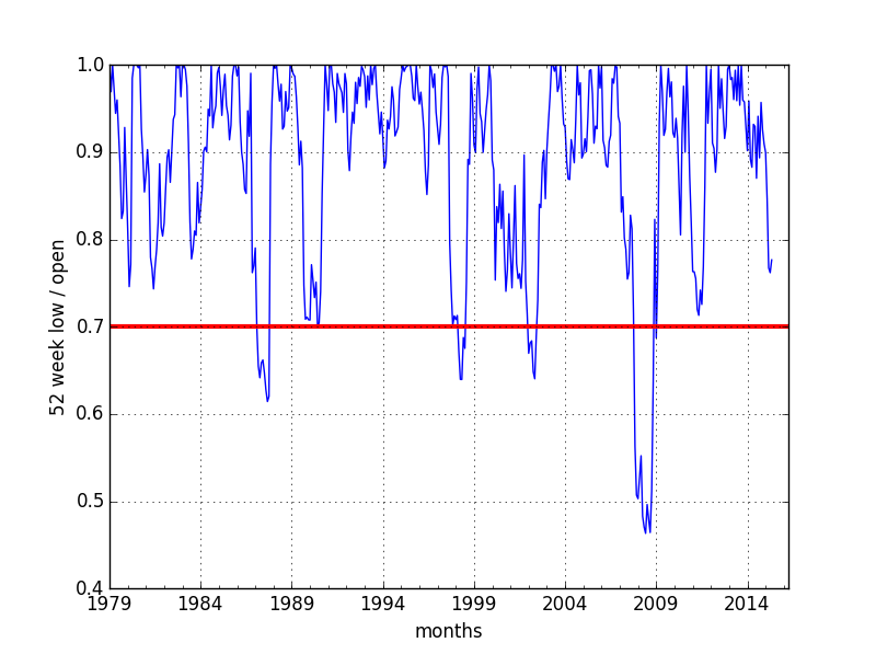
Finally, I plot the results versus a line at the 70% trigger level, which clearly shows four time frames when this occurred, including leading into 1987 and 2008. I could then have used Pandas to flag those time frames when the trigger hit and also compute the actual loss of principal (the ratio of closing value / opening value, capped at a max of 1.0). However at this point I wanted to eyeball the results and check them anyway, so I wrote the final DataFrame out to a csv file and dropped back to Excel. That’s actually a handy feature: it’s very both to pull data in from Excel and to write it out. Although I used a csv file for compatibility, Pandas can directly write excel formatted files as well.
#Plot out the low trigger versus the 70% of value trigger line
plt.figure(); trigger_monthly['Trigger_Value','combo'].plot(color='b'); plt.figure(); trigger_monthly['Trigger_Value','combo'].plot(color='b');
plt.axhline(y=0.7, linewidth=3, color='r')
plt.xlabel('months')
plt.ylabel('52 week low / open')
plt.show()

trigger_monthly.to_csv('triggerResults.csv')
Minimum Trigger Values and the 70% Trigger Level
If you’d like to see the full code, I posted it as a Github Gist at https://gist.github.com/ViennaMike/f953f531d5aaef071da22cdbec248794
Getting Started and Learning More
Python and the necessary libraries are much easier to install on Linux machines than on Windows, while on Macs I hear it’s a bit in between, as python comes pre-installed but it’s often not an up to date version. But regardless of your environment, I recommend you use the free Anaconda distribution of Python from Continuum Analytics. It’s a complete package with all the scientific python libraries bundled it. If Python has “batteries included,” Anaconda includes a whole electrical power plant. It also avoids library version inconsistencies or, on Windows, issues with installing underlying C based libraries.
The book on Pandas is Python for Data Analysis by Wes McKinney. It has lots of good examples that it walks you through. The website for Pandas is at http://pandas.pydata.org/ and the online documentation is quite good.
I recently also came across this blog post on the blogger’s top 10 features of Pandas and how to use them: Python and Pandas Top Ten.
The next time you need to wrangle some data, give Pandas a try.